
In my last article I show you guys how we can implement Polynomial Regression using python. In this article I’ll show you how we can implement Exponential Regression in python. In this article I’m going to show you 3 ways in which we can implement exponential regression in python. In the last I’m going to show you how the actual calculations work in calculating the values of optimal parameters in exponential regression.
This might be a long post, but believe me you are going to learn so much when you reach the end of the article. So hang tight!
Some real life examples of Exponential Growth:
(1) Microorganisms in culture.
(2) Spoilage of food.
(3) Human Population.
(4) Compound Interest.
(5) Pandemics Covid-19 :(
(6) Ebola Epidemic.
(7) Invasive Species
(8) Fire
(9) Cancer Cells
(10) Smartphone Uptake and Sale
The exponential function is given by :
where,
a = Shift value (on Y-axis)
b = Y-intercept / Multiplication factor
c = Base of the exponent
X = Input-features
f(X) = Output
The parameter b is called the y-intercept and c is called the base. Together, they completely determine the exponential function’s input-output behaviour.
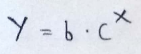
Here, first we are going to ignore a since it’s not that important(It just shifts value on the y-axis!!). So, our equation will be :
(1) Here you can notice that f(0) = b*c⁰ = b*1 = b. So we can say that when X = 0 the function returns us the value of y-intercept.
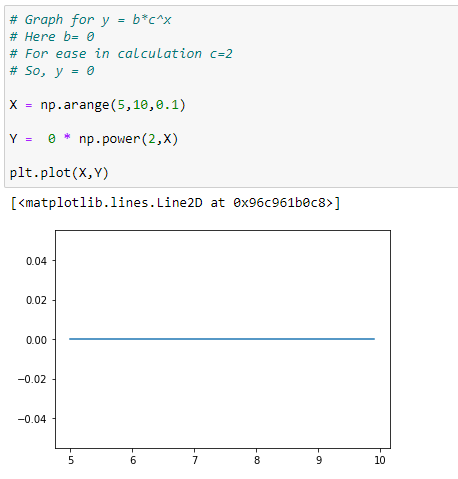
(2) When b=0 the function simplifies to f(x) = 0 or a constant function whose output is 0 for every input.
f(X) = 0*c^x = 0
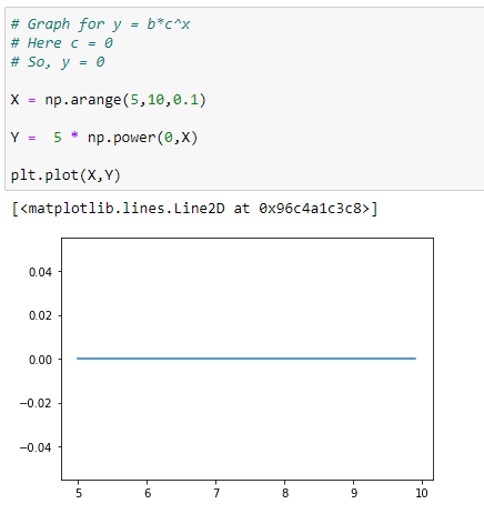
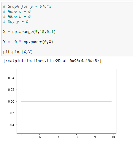
(3) When c=0 the function simplifies to f(x) = 0 or a constant function whose output is 0 for every input.
f(x) = b * 0^x = 0
(4) b = c = 0
f(x) = 0 * 0^x = 0
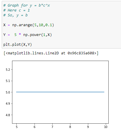
(5) When c = 1 we can see that f(x) = b, or a constant function whose output is b for every input.
f(x) = b * 1^x = b
What if we take negative base into account?
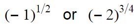
You can see that these formulas doesn’t make sense as nth root of a negative number is not-defined or imaginary in many cases. So here we are going to add some restrictions to our exponential function.
The base “C” of exponential function must be positive or zero.
Since we have already talked about base c = 0, from now on we are going to consider only positive bases.
Actual function :
Because we only work with positive bases , c^x is always going to be positive. So from that we can say that the the value of y or f(x) is either always positive or always negative, depending on the value of b.
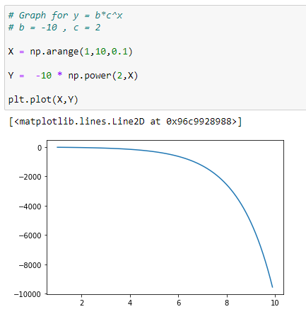
(1) positive b value return positive y value :
(2) negative b value returns negative y value :
Moving Forward,
The base c determines the rate of growth or decay :
(1) If 0<c<1 then then function decays as X increases. Smaller values of b leads to faster rates of decay.
Example :
(1/2)¹ > (1/2)² > (1/2)³
(1/4)¹ > (1/4)² > (1/4)³
Example :
(1/2)¹ = 0.5
(1/2)² = 0.25
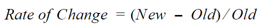
Rate of Change = (0.25–0.5)/0.5 = |-0.5| = 0.5
Example :
(1/4)¹ = 0.25
(1/4)² = 0.0625
Rate of Change = (0.0625–0.25)/0.25 =| -0.75| = 0.75
Why taking mod?
We know that negative sign represents decay. To find the actual rate we take the absolute values of it.
Here we can see that,
0.75(Rate of Change for 1/4)> 0.25(Rate of Change for 1/2)…
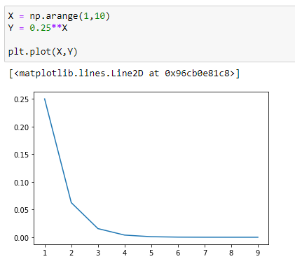
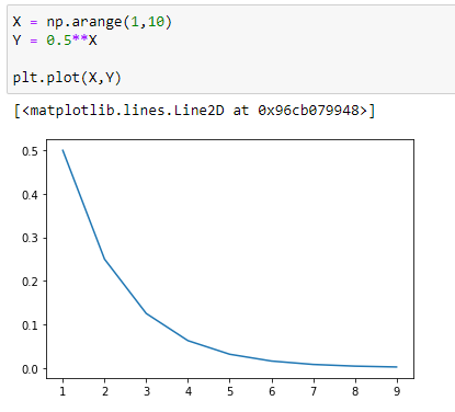
Okay so in conclusion we can see that, the smaller the value of base “c” the faster(greater) the rate of decay.
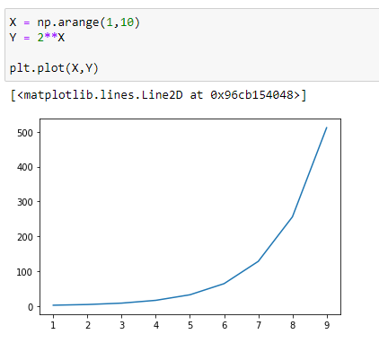
Let’s visualize it :
(1) y = 0.25^x
(2) y = 0.5^x
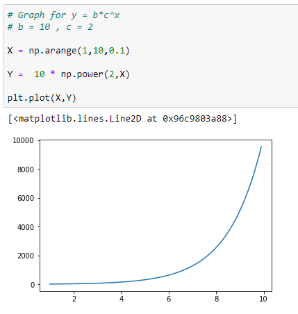
(2) If c > 1, the function grows as x increases.
2¹ > 2² > 2³
4¹ > 4² > 4³
Example :
2¹ = 2
2² = 4
Rate of Change = (4–2)/2 = 1
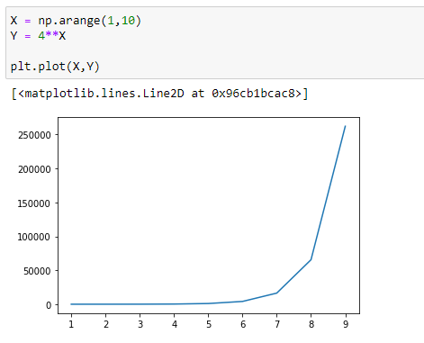
Example :
4¹ =4
4² = 16
Rate of Change = (16–4)/4 =4
Here we can see that,
4(Rate of change when c =4) > 1(Rate of Change When c=2)
So in conclusion, we can say that if c>1, the greater the value of base “c”, the faster the rate of growth.
Let’s visualize it :
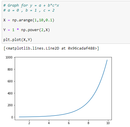
Remember we ignored the first parameter “a” from our function? Now it’s time it to get it back!!
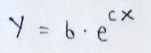
Our main exponential function is :
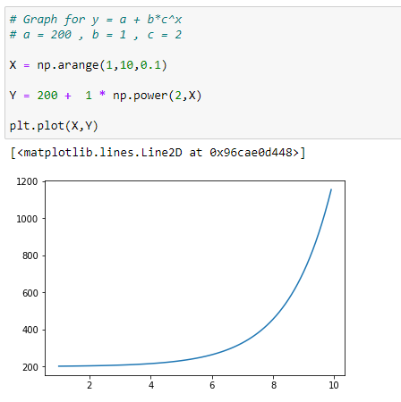
Here “a” is the shift value. It means that positive “a”value will shift our graphs that much units on +ve y axis and negative “a” will shift our graphs that much units on -ve y axis.
Let’s take an example :
(1) Without a :
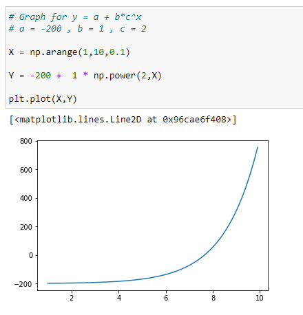
(2) With a = +200
(3) With a = -200
Exponential Functions We Generally See :
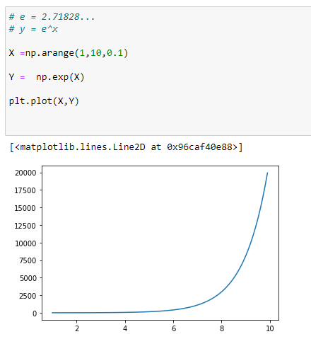
(1) Y = e^X
The Natural Log :
Why? Because we are going to use some of these rules in our derivation.
If you are taking a high school or college math class, you’ll likely cover natural logs. But the question comes in our mind that what is natural log? And what does the letter “e” means?
The natural log or ln is the inverse of e. The letter “e” represents a mathematical constant also known as the natural exponent. Like pi, e is a mathematical constant and has a set value. The value of e is equal to approximately 2.71828
e appears in many instances in mathematics, including scenarios about compound interest, growth equations, and decay equations. ln(x) is the time needed to grow to x, while e^x is the amount of growth that has occurred after time x.
Basic rules for natural log :
(1) Product rule :
ln(xy) = ln(x) + ln(y)
Example :
ln(8*6) = ln(8) + ln(6)
(2) Quotient Rule :
ln(x/y) = ln(x) — ln(y)
ln(8/3) = ln(8) — ln(3)
(3) Log of 1 :
ln(1) = 0
(4) log of e :
ln(e) =1
(5) Reciprocal Rule :
ln(1/x) = -ln(x)
ln(1/8) = ln(1) — ln(8) = -ln(8)
(6) Power rule :
ln(x^y) = y * ln(x)
ln(2³) = 3 * ln(2)
Okay..So before we move forward to the implementation of exponential equation I hope you already read my previous article on Linear Regression using normal function, since we are going to use almost the similar method to implement it.
In the last article we saw how we can derive the Normal Equation. So in this article we are going to solve the Simple…medium.com
Moving Forward to the implementation of exponential function in python.
Method 1 : Without Libraries / From Scratch:
Let’s first have a look at something we are working with.
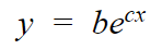
(1) Our function :
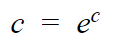
(2) Actual value of c :

(3) Function we’ll be working with in implementation :
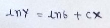
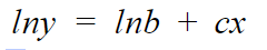
(4) Take natural log both sides :
(5) Matrix representation :
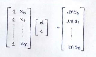
(6) Normal Equation :
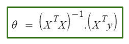
In the above equation :
θ : hypothesis parameters that define it the best.
X : input feature value of each instance
Y :Output value of each instance

Implementation using Normal Equation :
Let’s code :
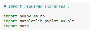
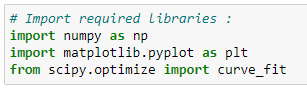
(1) Import required libraries :
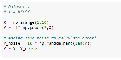
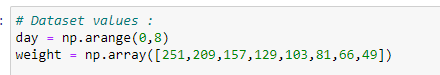
(2) Data points :
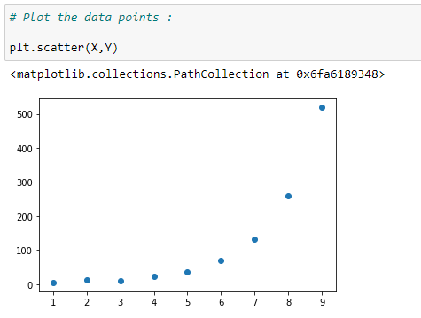
(3) Visualize the data :
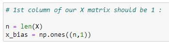
(4) Initialize 1st column of matrix X :
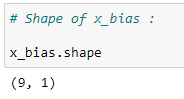
(4) Shape of x_bias :
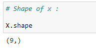
(5) Shape of X :
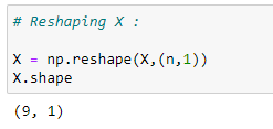
(6) For addition or appending data, matrices must be of same size. So reshaping X :
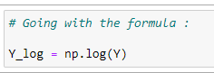
(7) Formatting data according to our formula :
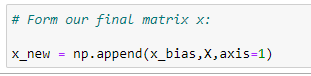
(8) Forming main matrix X :
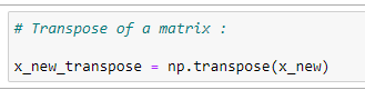
(9) Transpose of a matrix :
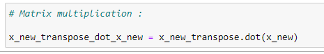
(10) Matrix multiplication :
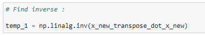
(11) Find inverse :
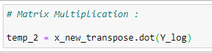
(12) Matrix Multiplication :
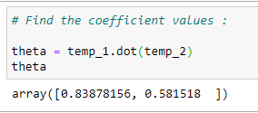
(13) Coefficient :
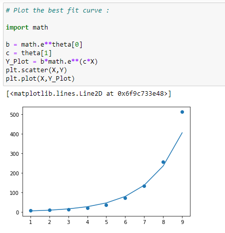
(14) Plot the best fit curve :
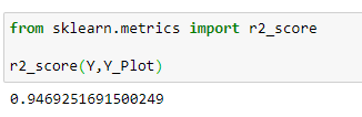
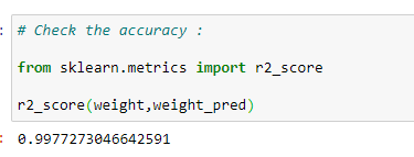
(15) Accuracy of model :
Disadvantage of Normal Equation :
(1) It’s slow if we are working with larger datasets. (Normally >100K)
Method 2 : Using Scipy Library
Here we’re going to implement exponential regression using scipy library. In the above method we had to find the optimal parameters using normal equation, but here scipy makes it easier. It returns us the parameters with just one line of code. Interesting isn’t it?
But It is always good to know the logic behind the calculations, right?
If you are reading this line then send “Hail Patrick_Star!! ” in response!! Let’s see how many of us made it this far!!!
Let’s code :
(1) Import required libraries :
(2) Data points :
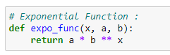
(3) Exponential function:
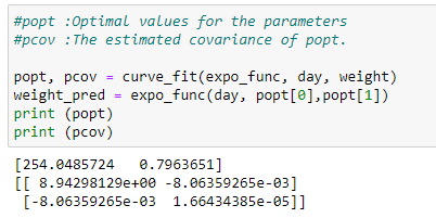
(4) Optimal parameters and covariance :
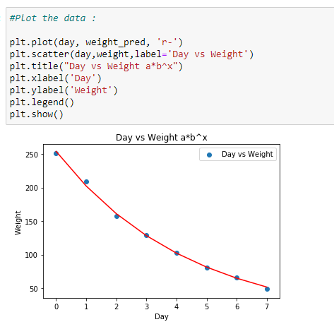
(5) Plot the data :
(6) Check the accuracy of model :
Putting it all together :
That was easy right. We just got our optimal parameters very easily, but have you ever wondered how the actual calculation works? If you are curious enough to know then I think you should definitely check the derivation of it. Otherwise, I hope you enjoyed this article and learned something new :)
Derivation of Exponential Regression Formula From Scratch :
Our function is :
Here notice that,
But to simplify the calculations, we generally write it as:
Our derivation will be based on :
Taking Natural log on both the sides :
Now, the above equation is similar to line equation,
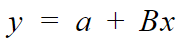
Where,
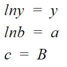
So, to derive the parameters values we will use our y = b+mx function and then replace it accordingly.
Check out this video for in-depth understanding of Simple Linear Regression
Let’s start by defining a few things:
1) Given n inputs and outputs.
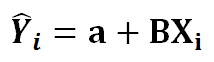
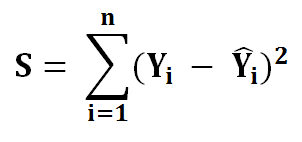
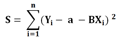
2) We define the line of best fit as…
3) Now we need to minimize the error function we named S…
4) Put the value of equation 2 into equation 3.
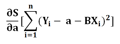
To minimize our error function, S, we must find where the first derivative of S is equal to 0 with respect to a and b. The closer a and b are to 0, the less total error for each point is. Let’s find partial derivative of a first.
Finding a :
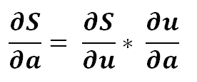
1 ) Find the derivative of S with respect to a..
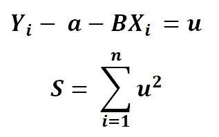
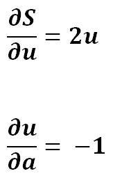
2 ) Using chain rule.. Let’s say ..
3) Using partial derivative..
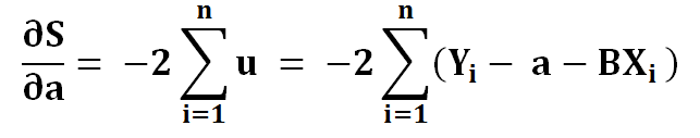
4) Expanding …
5) Simplifying…
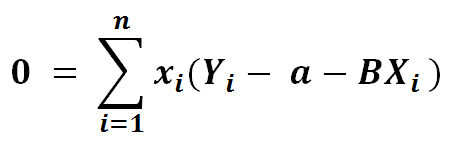
6) To find extreme values we put it to zero…
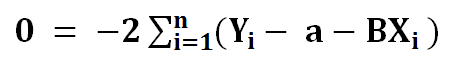
7) Dividing the left side with -2…..
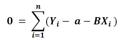
8) Now let’s break the summation in 3 parts..

9) Now the summation of a will be an….

10) Substituting it back in the equation…

11) Now we need to solve for a..

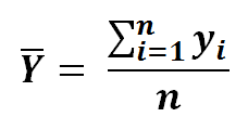
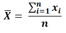
12) The summation of Y and x divided by n, is simply it’s mean..

We’ve minimized the cost function with respect to x. Now let’s find the last part which S with respect to b.
Finding B :
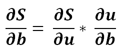
1 ) Same as we done with a..

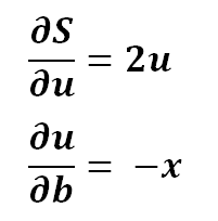
2) Finding the partial derivative…
3) Expanding it a bit..
4) Putting it back in the equation..
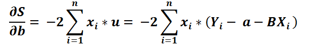
5) Let’s divide by -2 both sides..
6) Let’s distribute x for ease of viewing …

Now let’s do something fun!! Remember we found the value of a earlier in this article? Why don’t we substitute it? Well, let’s see what happens!!
7) Substituting value of a…


8) Let’s distribute the minus sign and x…

Well, you don’t like it? Let’s split up the sum into two sums…
9) Splitting the sum..

10) Simplifying…

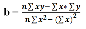
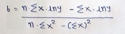
11) Finding B from it..

Great!! We did it!! We have isolated a and b in form of x and y. It wasn’t that hard, was it?
Still have some energy and want to explore it a bit!
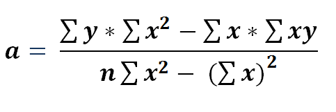
12 ) Simplifying the formula…
13) Multiplying numerator and denominator by n in equation 11…
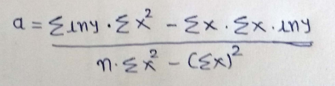
14) Now if we simplify the value of a using equation 13 we get…
Replacing our parameters :
From 13 ,
From 14,
Now we can easily find the regression curve.
For detailed explanation on this : Read this or Watch this
I hope you guys enjoyed it and learned something from it. If you really enjoyed it then hit the clap icon, that will encourage me to write such in-depth explanatory articles on various machine learning algorithms. I will keep posting such articles here and on by blog.
I regularly post my articles on : patrickstar0110.blogspot.com
All my articles are available on: medium.com/@shuklapratik22
I also post explanatory videos on my YouTube channel:
Here I will post some videos related to machine learning algorithms in detail. If you guys like these videos then…www.youtube.com
If you have doubts about anything in this article, feel free to contact me : shuklapratik22@gmail.com